Deep Dive into Qubits
Types of Qubits
There are different types of Qubits which vary in:
- Errors
- Scalability
- Use Case
Photonic Qubits
- Photonic Qubits utilise light particles, specifically photons, as the fundamental units of quantum information.
- They are manipulated by optical elements, such as prisms and silicon photonic chips, with beam-splitters and mirrors serving as quantum gates.
- Photonic Quantum Computing (PQC) allows for the encoding of quantum information in various ways, including through the polarisation of photons or their paths of travel.
- This technology is advantageous for its resilience to certain types of noise sources and the ability to travel long distances along existing fibre optic cables, supporting the idea of a quantum internet.
- However, it faces challenges like the need for quantum error correction and the requirement for cryogenic equipment for certain components.
Super Conducting Qubits
- Superconducting Qubits operate at critical low temperatures where resistance is nearly zero, allowing for the representation of current flowing in different directions as 0 and 1.
- These qubits are manipulated using electromagnetic pulses to control the magnetic flux, electric charge, or phase difference across specific areas of the superconducting circuit.
- They are known for their speed, simple gates, and high-quality operations but face challenges such as short lifespan, requiring extensive error corrections, and the need for cooling to very low temperatures.
- Superconducting qubits are used by companies like Google and IBM in their quantum computers, showcasing their potential for high-speed operations.
Trapped Ion Qubits
- Trapped ion qubits are based on the electronic and nuclear spin states of individual ions that are trapped and manipulated using electromagnetic fields. They can be implemented using ions like calcium, magnesium, and beryllium.
- Each ion acts as a qubit, and interactions between them are controlled using laser or microwave radiation. This radiation is used to execute logic gates by coupling the ground states of the ion to the motion of the ions, inducing entanglement. This allows the system to perform more complex computations.
- Trapped-ion qubits have particularly long coherence times, which is how long a system maintains its quantum state. It can be orders of magnitude higher than in superconducting qubits, reducing error correction requirements. This allows quantum information to be stored and manipulated for longer, allowing for high-fidelity operations.
- While trapped-ions themselves don’t need to be super-cooled during operation and can be at room temperature, the surrounding machinery does need temperature control to maintain a high vacuum and stable electromagnetic field. The heat from the lasers also needs to be cooled.
Topological Qubits
- Topological qubits are a highly experimental type of qubit that use a unique form of particle known as anyons. These qubits are made resistant to noise and errors through their braided nature, requiring far fewer qubits to achieve utility .
- They operate in a non-Abelian quantum phase of matter known as a topological state of matter, which was largely theoretical until recent breakthroughs by researchers from Microsoft and Quantinuum proved it was possible.
- Topological quantum computers may still require super=cooling like superconducting qubits, as the topological state of matter is very delicate and could be easily disturbed by thermal fluctuations. Coherence times and scalability for these qubits are not yet fully understood.
Nitrogen Vacancy Centre Qubits
- Nitrogen Vacancy (NV) centres are created by replacing a single carbon atom in a diamond’s atomic lattice with a nitrogen atom and leaving a neighbouring lattice node empty. This creates a flaw, or blemish, in an otherwise super-pure atomic structure.
- In this setup, electrons occupy orbitals inside the vacancy of the NV centre while the NV centre’s electronic spins react with the nuclear spin of some of the carbon atoms nearby. Both the NV centre and the adjacent carbon atoms function as qubits, and the diamond lattice keeps them stationary and entangled.
- These qubits—called solid-state spin qubits—are limited since the system can only have as many qubits as there are neighbouring carbon atoms. NV centres are difficult to control, which means they might not be as scalable as other options. However, they can operate at room temperature, which is a significant advantage.
- Researchers have entangled an NV centre’s electronic spin with the spins of nine nearby nuclei, indicating promising progress in this burgeoning technology.
Issues with Qubits:
Qubits are highly sensitive are sensitive to many factors are cause errors.
- Temperature
- Light
- Vibrations
- Other qubits
- Cosmic rays
These factors are called as Noise and can lead to decoherence of qubits .i.e
- Relaxation: Switching from high level to low level state
- Dephasing: Loss of Phase information
Good Quantum Computer
The Da Vincenzo’s criteria for a good QC is:
- Well characterised and scalable qubits
- Initialisation Qubits
- Long coherence items
- Universal set of gates
- Efficiently measurable
Swamp test
Fidelity measures how close two quantum states are to each other and is given by:
\[\text{fidelity}=|\bra{\psi}\ket{\phi}|^2\]Swamp Test provides the fidelity. We can derive the equation from the below circuit for two bit. 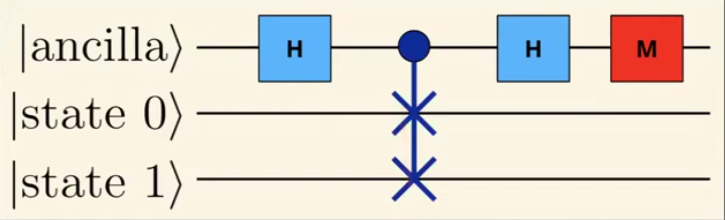
The circuit can be mathematically shown as:
\[\ket{0}\ket{state 0}\ket{state 1}\]After applying H gate to ancilla qubit:
\[\frac{1}{\sqrt{2}}(\ket{0}\ket{state 0}\ket{state 1} + \ket{1}\ket{state 0}\ket{state 1})\]Now we apply controlled swap gate which swaps state 0 and state 1. After swap gate we also apply H gate :
\[\frac{1}{2}[(\ket{0}\ket{state 0}\ket{state 1} + \ket{1}\ket{state 1}\ket{state 0}) \ + \ (\ket{0}\ket{state 1}\ket{state 0} + \ket{1}\ket{state 1}\ket{state 0})]\] \[\frac{1}{2}[(\ket{0}\ket{state 0}\ket{state 1} + \ket{1}\ket{state 1}\ket{state 0}) \ + \ (\ket{0}\ket{state 1}\ket{state 0} + \ket{1}\ket{state 1}\ket{state 0})]\]Finally when we measure:
\[\text{probability(ancilla=0)} = \frac{1}{2}(|\bra{state0}\ket{state1}|^2+1)\]in terms of fidelity:
\[\text{probability(ancilla=0)} = \frac{1}{2}(\text{fidelity}+1)\]Code (Noise)
# 1. Depolarizing Noise
qubits = cirq.NamedQubit.range(2, prefix = 'q')
circuit = cirq.Circuit()
circuit.append(cirq.H(qubits[0]))
circuit.append(cirq.CNOT(qubits[0], qubits[1]))
circuit.append(cirq.measure(qubits))

# Apply Noise
noise = cirq.depolarize(0.05)
simulator = cirq.Simulator()
result = simulator.run(circuit.with_noise(noise), repetitions = 1000)

hist = cirq.plot_state_histogram(result, plt.subplot(), title = '5% Depolarization', xlabel = 'States', ylabel = 'Occurrences', tick_label=binary_labels(2))
plt.show()
To the above code you would see the below results: 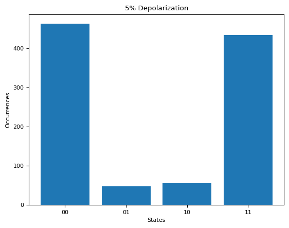
For a Bell State of \(\frac{1}{\sqrt{2}} (\ket{00}+\ket{11})\) only \(\ket{00}\) and \(\ket{11}\) is expected.
# 2. Swamp Test
q0 = cirq.NamedQubit('state 0')
q1 = cirq.NamedQubit('state 1')
ancilla = cirq.NamedQubit('ancollia')

circuit_0 = cirq.Circuit()
circuit_0.append(cirq.I(q0))
circuit_1 = cirq.Circuit()
circuit_1.append(cirq.X(q1))
circuit = circuit_0 + circuit_1

#Swamp Test Cirquit
circuit.append(cirq.H(ancilla))
circuit.append(cirq.CSWAP(ancilla, q0, q1)
circuit.append(cirq.H(ancilla))
circuit.append(cirq.measure(ancilla))

# Simulate the results
simulator = cirq.Simulator()
result = simulator.run(circuit, repetitions=1000)

# Fidelity
prob_0 = np.sum(result.measurements['anc']) / len(result.measurements['anc'])
fidelity = 1 - 2*prob_0